Data Storage

The data storage layer is a fundamental component of the BOS infrastructure, serving as the backbone for efficient data handling, retrieval, and long-term system scalability. The design of this layer must accommodate large volumes of heterogeneous data while ensuring high performance, reliability, and ease of integration with various applications. To achieve these objectives, a structured approach was adopted, incorporating trade-offs and design patterns that optimize both storage efficiency and system modularity. A key consideration in the design of the data storage layer is the separation of data and metadata management. By employing dedicated databases for each, it becomes possible to address the distinct challenges posed by time series data storage and metadata organization independently. This separation enhances system performance by allowing each database to be optimized for its specific function—time series databases are tailored for handling high-frequency sensor data, while metadata repositories provide structured and contextualized information about the monitored assets, devices, and data streams. The advantages of this approach extend beyond performance optimization. Dedicated databases improve system maintainability, facilitate scalable data processing, and enable flexible data access patterns. Furthermore, this design allows for seamless integration with analytical and decision-support applications, ensuring that energy management insights can be efficiently extracted and utilized. As a result, the implemented data layer consists of two primary components: time series storage and metadata storage. The following sections provide a detailed discussion of these concepts and their implementation within the BOS framework.

Time series data storage

A time series is a sequence of data points indexed in time order, typically measured at successive points in time, spaced at uniform intervals. In the context of building automation, time series data is crucial for monitoring and controlling various systems, such as HVAC, lighting, and security.

In the case study analyzed, the amount of data generated is massive, with almost 1.5 Billions of records from 2014 to July 2024, the polito infrastructure processes and ingests an average of 500,000 data points per day at a rate of 21,000 per hour. Figure 1 illustrates the growth of data from 2014 to the present.

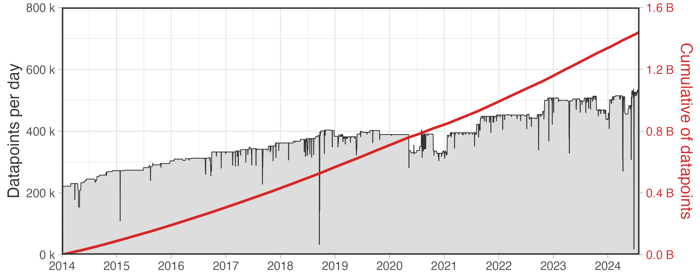Figure 1: Acquired data points from 2014 to 2024. On the left axis the number of measurements processed per day while on the right axis the cumulative number of measurements.

Time-series data accumulates very quickly, and challenges related to the storage of such data in traditional relational data sources, lead to the development of more efficient databases designed to handle such scale efficiently [McBride et al., 2020]. Although processing such volume of data is the main challenge, there are some other aspects to be considered when dealing with time series. Such data tends to be accessed in sequential order, are rarely updated and for many applications the data can be aggregated or discarded after a suitable interval of time [McBride et al., 2020]. This is the reason behind the development of databases specifically designed to manage time-stamped or time-series data, known as TSDB. These databases leverage time-oriented optimizations (e.g., batching data or data compression) to enhance storage and computational operations, efficiently handling large numbers of transactions in very short periods. Examples of time-series databases include InfluxDB, Cassandra, OpenTSDB, and TimescaleDB. Although every database has its own characteristics and performances, the right choice for a database always depends on the case study. For this specific case study, TimescaleDB was selected due to its capability to query time-series through SQL language. Its SQL-like features make it accessible to those who are already accustomed to working with PostgreSQL relational database, i.e. the existing Operations and Maintenance (O&M) staff, allowing easier maintenance of the infrastructure in the long term.

Data model

While there is a general notion of how time series data is structured, different solutions offer different models for representing this data. Variations may occur in how time is represented, data types are supported, and how metadata is handled. In particular, there are two main ways to store time series:

Wide table model In the wide table model, a time series is a table keyed by time, with multiple columns representing different metrics. This model is suitable when a single sensor measures several parameters simultaneously and the acquisition timestamp is synchronized and known a priori. However, it can create bottlenecks in database scalability since it is required to know in advance the number of variables and sensors. This approach is impractical for a large and heterogeneous monitoring infrastructure, as data may be collected at different timestamps, the number of sensors is undefined. Additionally, if measurements do not share the same timestamp, the table may become sparse when new measurements are added.
Narrow table model To solve this issue, the narrow table model may be adopted. This data model represents a time series as a table keyed by time with a single column of values and eventually tags related to the sensors. This model allows for the storage of observations not aligned in time or collected with heterogeneous timestamps, however the downside of this approach is that the table may grow very quickly and data query may not be straightforward.

As TimescaleDB does not impose its own model of a time series, supporting both narrow and wide table models, the long data format was chosen for the polito case study, due to its flexibility and scalability when applied to large monitoring infrastructures. The chosen table structure for storing time series data consists of four columns: time, meter_id, value, and tag as illustrated in Figure 2 on the left. Each record is uniquely identified by a composite primary key consisting of the time and meter_id. This design allows for the ingestion of time series with varying timestamps but ensures that only one measurement per meter id can be written at any given time, thus maintaining data consistency. The value column is a floating point and represent the measurement while the tag column is an additional metadata that can be added to tag the quality of the single measurement. Raw data is stored with infinite data retention, meaning there is no retention policy, thus ensuring all raw data remains accessible.

Figure 2: Graphical representation of employed time-series data model through the application of hyper-tables and continuous aggregates concepts.

Storage and query optimization strategies

Although the narrow table model can be efficient for data modeling, it is crucial to optimize performance in terms of data retrieval, query execution, disk space usage, and data accessibility. Referring to Figure 1, the number of observations at a one-minute timestamp recorded every day is in the order of hundreds of thousands, which implies that the table contains an enormous number of rows. With the aim to optimize the database the following strategies were adopted.

Hypertables

TimescaleDB allows to enhance the query performance by transforming the traditional SQL table into a hyper-table (Figure 2 in the middle). This approach consists in automatically partition data by time, allowing for efficient storage and querying of time-series data. By letting the system manage partitioning into manageable chunks—each representing a specific time range—this strategy simplifies the database architecture. From a performance standpoint, smaller chunks improve query speed for recent or time-bounded data, while larger chunks can slow down inserts and increase query latency.

In the specific implementation presented in this thesis, the hyper-table called monitoring_data was created with 30 days chunks. This means that all incoming time-series data are automatically grouped into partitions spanning 30 days each. Choosing a 30-day chunk size strikes a balance between query performance, storage efficiency, and system maintenance overhead according to the amount of data ingested every day and the overall system memory. It ensures that each partition contains a sufficient amount of data to benefit from bulk processing and compression, without becoming too large to manage efficiently. Therefore, a 30-day duration offers a pragmatic compromise—large enough to minimize the number of partitions, yet small enough to maintain high query performance and efficient data eviction or retention policies. To further enhance data access an index was created on the meter_id column to enhance query performance when querying subsets of UUIDs. The SQL code used to create the hyper-table is reported below:

CREATE TABLE monitoring_data
(
    time     TIMESTAMPTZ NOT NULL DEFAULT NOW(),
    value    FLOAT       NOT NULL,
    meter_id INTEGER     NOT NULL,
    tag      TEXT        NOT NULL,
    CONSTRAINT fk_meter
        FOREIGN KEY (meter_id)
            REFERENCES monitoring_meter (id)
            ON DELETE RESTRICT,
    PRIMARY KEY (time, meter_id)
);

SELECT create_hypertable('monitoring_data', 'time',
                         if_not_exists => TRUE,
                         migrate_data => TRUE,
                         create_default_indexes => TRUE,
                         chunk_time_interval => interval '30 day');

Continuous Aggregates

Another optimization performed on the database is related to the data retrieval pattern. In the analyzed case study, data access typically occurs at aggregation intervals greater than one minute, such as 15-minute intervals, as shown on the right in Figure 2. This choice aligns with both regulatory standards and research practices in energy monitoring and analysis, where 15-minute intervals are commonly used to balance temporal resolution and data storage efficiency [Albert et al., 2013; OpenADR, 2012; ENTSO-E, 2023].

For this purpose, another key feature of TimescaleDB, continuous aggregation, was exploited. Continuous aggregates allow the database to automatically refresh aggregated data as new information becomes available, maintaining up-to-date insights without requiring manual intervention.

In the proposed data structure, a continuous aggregation is performed and refreshed every 15 minutes, alongside the creation of additional columns containing summary statistics such as average (avg_value), minimum (min_value), maximum (max_value), and sum (sum_value) of the values contained in each time bucket.

Figure 3 shows how an electrical load time series can be represented through the continuous aggregate with a 15-minute time bucket. Figure 3(a) at the top shows the raw data acquired from a photovoltaic electrical power meter with 1-minute sampling frequency. Figure 3(b) at the bottom shows how the same time series is transformed by the continuous aggregate table with 15-minute aggregation. Different continuous aggregate tables were created, namely a 15-minute (monitoring_data_15m), 1-hour (monitoring_data_1h), and 1-day (monitoring_data_1d) aggregation.

Continuous aggregate example Figure 3: Example showing how the raw 1-minute sampling frequency time series (a) is processed by the TimescaleDB continuous aggregate function and transformed into a 15-minute sampling frequency time series (b).

Compression

Finally, to optimize disk space usage, a compression policy was implemented on both the raw data hypertable and the continuous aggregates table for data older than 5 years. Since access to older data is infrequent, applying compression significantly reduces storage space and related costs. By compressing older data, the database maintains efficient long-term data management without compromising performance. This strategy is essential for managing vast datasets and reducing overall storage expenses, ensuring that the system remains scalable and cost-effective over time.